
A Lesson in Unit Testing
Quite some time back, I wrote a Python library for simple clustering tasks. Back in the day, I only needed K-Means clustering. But I decided I would add hierarchical clustering as well as it could come in handy later on.
Turns out I messed up the unit tests, and the hierarchical clustering algorithm. But the error went unnoticed as the unit-tests were not testing one obvious fact:
Are all the elements from the input present in the output? And only those from the input?
The main cause of this error is because the way I obtained the expected values was complete heresy! I ran the test run on random values, and simply copy/pasted the results into the expected values. Of course now the test passed, with the important fact that the tests were testing against the wrong values!
In order to fix address this, I first need some proper test values. So now I do what I should have done in the first place: Manually step through the algorithm. This article contains my scribbles which I will use as a "mental strut".
Hierarchical Clustering
We will start of with a sample of non primitive data types. In this case points on a two-dimensional plane. As distance function we will use the euclidian distance. And, for the first step through, we will use single linkage between clusters. The same scenario will be played through with complete- and uclus-linkage later on. As overall method, we will use a bottom-up approach.
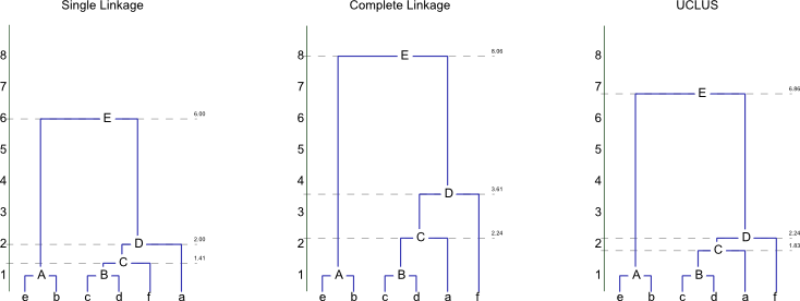
The three aproaches will result in the following dendograms:
Initial Step
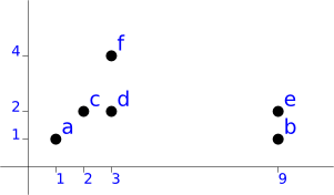
So we have the following points:
a (1, 1)
b (9, 1)
c (2, 2)
d (3, 2)
e (9, 2)
f (3, 4)
Note
To keep the matrix table more readable, individual points are written in lower-case, while clusters are written in upper-case!
This results in the following initial distance matrix. We will mark the diagonal with an x as we're not interested in comparing a point with itself. Equally, we are only interested in the absolute distance. So we only need the values for pairs on ons side of the diagonal.
| a | b | c | d | e | f | |
|---|---|---|---|---|---|---|
| a | x | 8.00 | 1.41 | 2.24 | 8.06 | 3.61 |
| b | x | 7.07 | 6.08 | 1.00 | 6.71 | |
| c | x | 1.00 | 7.00 | 2.24 | ||
| d | x | 6.00 | 2.00 | |||
| e | x | 6.32 | ||||
| f | x |
Single Linkage
First Step
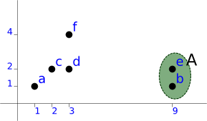
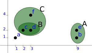
With this matrix, we see that the first candidates are [b, e] and [c, d]. We'll pick [b, e] as firt cluster (A):
a (1, 1)
A (9, 1), (9, 2) level=1.00
c (2, 2)
d (3, 2)
f (3, 4)
| a | A | c | d | f | |
|---|---|---|---|---|---|
| a | x | 8.00 | 1.41 | 2.24 | 3.61 |
| A | x | 7.00 | 6.00 | 6.32 | |
| c | x | 1.00 | 2.24 | ||
| d | x | 2.00 | |||
| f | x |
Second Step
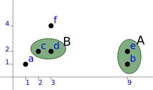
The next candidate is [c, d] as B:
a (1, 1)
A (9, 1), (9, 2) level=1.00
B (2, 2), (3, 2) level=1.00
f (3, 4)
Giving us:
| a | A | B | f | |
|---|---|---|---|---|
| a | x | 8.00 | 1.41 | 3.61 |
| A | x | 6.00 | 6.32 | |
| B | x | 2.00 | ||
| f | x |
Third Step
Then [f, B] as C:
a (1, 1)
A (9, 1), (9, 2) level=1.00
C (3, 4), ((2, 2), (3, 2) level=1.00) level=2.00
Resulting in:
| a | A | C | |
|---|---|---|---|
| a | x | 8.00 | 1.41 |
| A | x | 6.00 | |
| C | x |
Fourth Step
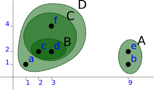
Then [a, C] as D:
A (9, 1), (9, 2) level=1.00
D (1, 1), ((3, 4), ((2, 2), (3, 2) level=1.00) level=2.00) level=1.41
Resulting in:
| A | D | |
|---|---|---|
| A | x | 6.00 |
| D | x |
Which gives us the final cluster E with a level of 6.00.
The end-result is the following dendogram:
               E
               |
   +-----------+-----------+
   |                       |
   |                       D
   |                       |
   |                 +-----+-----+
   |                 |           |
   |                 C           |
   |                 |           |
   |            +----+----+      |
   |            |         |      |
   A            B         |      |
   |            |         |      |
+--+--+      +--+--+      |      |
|     |      |     |      |      |
e     b      c     d      f      a
Complete Linkage
Initial distance matrix for reference:
| a | b | c | d | e | f | |
|---|---|---|---|---|---|---|
| a | x | 8.00 | 1.41 | 2.24 | 8.06 | 3.61 |
| b | x | 7.07 | 6.08 | 1.00 | 6.71 | |
| c | x | 1.00 | 7.00 | 2.24 | ||
| d | x | 6.00 | 2.00 | |||
| e | x | 6.32 | ||||
| f | x |
First Step
First iteration is identical, but distance matrix has different values. The subsequent steps will be displayed without aditional explanation, the idea is the same as above, simply using a different linkage function.
| a | A | c | d | f | |
|---|---|---|---|---|---|
| a | x | 8.06 | 1.41 | 2.24 | 3.61 |
| A | x | 7.07 | 6.08 | 6.71 | |
| c | x | 1.00 | 2.24 | ||
| d | x | 2.00 | |||
| f | x |
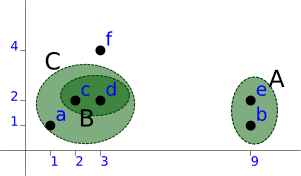
Second Step
| a | A | B | f | |
|---|---|---|---|---|
| a | x | 8.06 | 2.24 | 3.61 |
| A | x | 7.07 | 6.71 | |
| B | x | 2.24 | ||
| f | x |
Third Step
Note
We now have to make a choice. I have not yet decided on how to handle this situation to have a detereministic behaviour. My current train of thought is using python sets as data-structure which is unordered. So the algorithm could return either one here.
For a demonstration, we'll pick [Ba] as to have a different result from sinle linkage...
This will give us:
| C | A | f | |
|---|---|---|---|
| C | x | 8.06 | 3.61 |
| A | x | 6.71 | |
| f | x |
Fourth Step
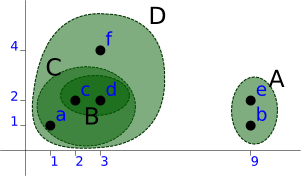
And finally
| D | A | |
|---|---|---|
| D | x | 8.06 |
| A | x |
The end-result is the following dendogram:
               E
               |
   +-----------+-----------+
   |                       |
   |                       D
   |                       |
   |                 +-----+-----+
   |                 |           |
   |                 C           |
   |                 |           |
   |            +----+----+      |
   |            |         |      |
   A            B         |      |
   |            |         |      |
+--+--+      +--+--+      |      |
|     |      |     |      |      |
e     b      c     d      a      f
Uclus
Initial distance matrix for reference:
| a | b | c | d | e | f | |
|---|---|---|---|---|---|---|
| a | x | 8.00 | 1.41 | 2.24 | 8.06 | 3.61 |
| b | x | 7.07 | 6.08 | 1.00 | 6.71 | |
| c | x | 1.00 | 7.00 | 2.24 | ||
| d | x | 6.00 | 2.00 | |||
| e | x | 6.32 | ||||
| f | x |
As in complete linkage, the first iteration is identical, but distance matrix has different values. So we will not go into too much detail and will skip the visualisations.
| a | A | c | d | f | |
|---|---|---|---|---|---|
| a | x | 8.03 | 1.41 | 2.24 | 3.61 |
| A | x | 7.04 | 6.04 | 6.52 | |
| c | x | 1.00 | 2.24 | ||
| d | x | 2.00 | |||
| f | x |
| a | A | B | f | |
|---|---|---|---|---|
| a | x | 8.03 | 1.83 | 3.61 |
| A | x | 6.54 | 6.52 | |
| B | x | 2.12 | ||
| f | x |
| C | A | f | |
|---|---|---|---|
| C | x | 7.04 | 2.24 |
| A | x | 6.52 | |
| f | x |
And finally
| D | A | |
|---|---|---|
| D | x | 6.86 |
| A | x |
The end-result is the following dendogram:
               E
               |
   +-----------+-----------+
   |                       |
   |                       D
   |                       |
   |                 +-----+-----+
   |                 |           |
   |                 C           |
   |                 |           |
   |            +----+----+      |
   |            |         |      |
   A            B         |      |
   |            |         |      |
+--+--+      +--+--+      |      |
|     |      |     |      |      |
e     b      c     d      a      f
